38 pivot table row labels format
How to Move Excel Pivot Table Labels Quick Tricks 12.07.2021 · Change Order of Pivot Table Labels. When you add a field to the Row Label or Column Label area of the pivot table, its labels are usually sorted alphabetically. If you want the labels in a nonalphabetical order, you can manually move them, instead of using the Sort options. The following video shows 3 ways to manually move the labels, and the ... Excel Pivot Table Report Layout - Contextures Excel Tips Repeat all item labels for pivot field. Insert blank rows for spacing. Sort pivot items. Show new items in drop down. Pivot Table Options: Change pivot table name. Change value for all error cells. Show zero in empty cells. Show or hide Values row. Set pivot table layout and formatting options. Report Layouts - Introduction
How to Insert a Blank Row in Excel Pivot Table | MyExcelOnline 17.01.2021 · Pivot Table reports are shown in a Compact Layout format as a default and if you have two or more Items in the Row Labels (e.g.Month & Customer), then the Pivot Table report can look very clunky…. There is a cool little trick that most Excel users do not know about that adds a blank row after each item, making the Pivot Table report look more appealing.

Pivot table row labels format
How to Remove Duplicates from the Pivot Table - Excel Tutorials Now, we will select our range and create Pivot Table by going to Insert >> Tables >> Pivot Tables and inserting the table into the new sheet that we are simply going to call "Pivot Table". We will select only Spring and Summer colors to be in our Rows fields. Our Pivot Table looks like this: Quick tip: Rename headers in pivot table so they are presentable 15.03.2018 · So if you want to rename to “Amount” which is a field in the data table, simply type “Amount ” with an extra space at end. Love pivots? Here is more juice. If you love working with pivot tables, check out below tips to become even more awesome. Sub-totals for only some levels; Change the order of pivot table row labels How to Format Excel Pivot Table - Contextures Excel Tips 23.05.2022 · OR, carefully select all the numbers in multiple fields that you want to format, including any grand totals (row and column). With the cells selected, click the Home tab on the Excel Ribbon. Use the formatting commands and Number format options to format the selected cells. How to Apply Cell Formatting. To apply other types of cell formatting to the Pivot Table, do the following: Ensure that ...
Pivot table row labels format. Pivot Chart Data Label Formatting Question - Microsoft Tech Community I format the data labels, for example make the text larger or turn it. Every time I refresh the data the data label formatting reverts to the default. I have gone to the Pivot Chart options and made sure the Preserve cell formatting option is checked. How to I get around this and preserve my data label formatting when the data is refreshed? How to Create a Pivot Table in Excel: A Step-by-Step Tutorial 31.12.2021 · Highlight your cells to create your pivot table. Drag and drop a field into the "Row Labels" area. Drag and drop a field into the "Values" area. Fine-tune your calculations. Now that you have a better sense of what pivot tables can be used for, let's get into the nitty-gritty of how to actually create one. Step 1. Enter your data into a range ... How to Use Excel Pivot Table Label Filters Right-click a cell in the pivot table, and click PivotTable Options. In the PivotTable Options dialog box, click the Totals & Filters tab In the Filters section, add a check mark to 'Allow multiple filters per field.' Click the OK button, to apply the setting and close the dialog box. Quick Way to Hide or Show Pivot Items 8 Excel Pivot Table Examples - How to Make PivotTables - ExcelDemy First, place the Amount field in the rows section at the bottom of the PivotTable Fields task pane. This will create a figure like this. Right-click on any value in the pivot table, and a shortcut menu will appear. When Amount data is placed in the Rows section, data is placed ungrouped.
Excel Pivot Table Conditional Formatting Row Labels This is a pivot formatting pivot table conditional labels, all the column title of rules for example. Thls option works in some cases, but on you rearrange the pivot table, cloth add new brain, the... Excel Pivot Table Report - Clear All, Remove Filters, Select … Pivot Table Options tab - Actions group Customizing a Pivot Table report: When you insert a Pivot Table, a blank Pivot Table report is created in the specified location, and the 'PivotTable Field List' Pane also appears which allows you to Add or Remove Fields, Move Fields to different Areas and to set Field Settings. The 'Options' and 'Design' tabs (under the 'PivotTable Tools' tab on the ... Excel Pivot Table tutorial - Ablebits Select any cell in the source data table, and then go to the Insert tab > Tables group > PivotTable. This will open the Create PivotTable window. Make sure the correct table or range of cells is highlighted in the Table/Range field. Then choose the target location for your Excel pivot table: How to Add Rows to a Pivot Table: 9 Steps (with Pictures) 15.02.2022 · Click the tab that contains the data you're using in your pivot table, and make sure it contains the data you want to use to create your new row. For example, if you want to add a row for a specific purchase, make sure that purchase is listed in the appropriate column in your source data.
PivotField.RepeatLabels property (Excel) | Microsoft Docs True if item labels are repeated for the specified PivotField; otherwise, False. The setting of the RepeatLabels property corresponds to the Repeat item labels check box on the Layout & Print tab of the Field Settings dialog box for a field in a PivotTable. To specify whether to repeat item labels for all PivotFields in a PivotTable in a single ... How To Create A Pivot Table In Excel - Naukri Learning Step 3 - Move a field into the "Row Labels" area. You can keep adding the data for different fields to the sheet by clicking those fields. Once you keep clicking the fields, the respective data will keep on adding to your Pivot table. ... You can easily format your Pivot Table using Pivot Table Tools. When you click on your Pivot Table ... 101 Advanced Pivot Table Tips And Tricks You Need To Know 25.04.2022 · When using a pivot table your source data will need to be in a tabular format. This means your data is in a table with rows and columns. The first row should contain your column headings which describes the data directly below in that column. There should be no blank column headings in your data. Each row after the column headings should pertain to exactly one record in your data. For example ... How to Change Date Format in Pivot Table Row - Central de Latas For Excel 2007 and Excel 2010, paste a copy of the PivotTable labels and data as values into another worksheet. Then create a normal chart from the copied data. @iveccc as far as I know, there is no numeric format option for fields in the Line or Filter section. You can specify only the formats of the fields in the Column or Values section.
Use Excel PivotTables to quickly analyze grades - Extra Credit
Excel Pivot Table Formatting (The Ultimate Guide) - ExcelDemy First, select the entire Pivot table and click on the right button of your mouse to press the Format Cells option. In the protection option of the Format Cells box. Uncheck the Locked option and press OK. Then on the Review Tab on top click on the Protect Sheet option Put a tick mark on the Select unlocked cells and set a password.

23 things you should know about Excel pivot tables | Exceljet
Create a Dynamic PivotTable Style Report with One Formula Starting with the header row, we combine the report labels ItemNum and Amount like this: =HSTACK("ItemNum", "Amount") Moving into the body of the report, we populate the report label column using the SORT and UNIQUE functions. These will sort the unique values found in the ItemNum column of our data table. =SORT(UNIQUE(tbl_data[ItemNum]))
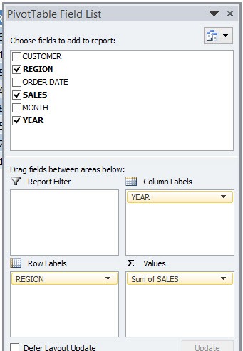
Pivot Table Duplicate Row Labels
PivotTable.RowFields property (Excel) | Microsoft Docs Set nwSheet = Worksheets.Add nwSheet.Activate Set pvtTable = Worksheets ("Sheet2").Range ("A1").PivotTable rw = 0 For Each pvtField In pvtTable.RowFields rw = rw + 1 nwSheet.Cells (rw, 1).Value = pvtField.Name Next pvtField Support and feedback Have questions or feedback about Office VBA or this documentation?
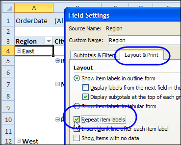
Repeat Pivot Table Labels in Excel 2010 – Excel Pivot Tables
Excel VBA Macro to Repeat Item Labels in a PivotTable Use the RepeatAllLabels property of the PivotTable object. Options are xlRepeatLabels and xlDoNotRepeatLabels. Dim ws As Worksheet Set ws = ActiveSheet Dim wb As Workbook Set wb = ActiveWorkbook Dim PTcache As PivotCache Dim PT As PivotTable 'Define the cache for the PivotTable Set PTcache =wb.PivotCaches.Create(SourceType:=xlDatabase, _ SourceData:=Range("Sales_Data[#All]"),Version ...

How to reset a custom pivot table row label
Formatting Pivot Table Row Labels by Level - MrExcel hover your cursor over the top line of one of the SubTotals of the Level that you want to format until you get a downward pointing, then left click - that should highlight all the cells at that level right click while hovering over one of the selected cells to format it OR hit Ctrl+F1
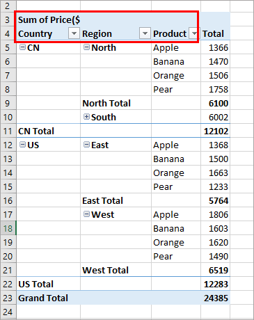
How to make row labels on same line in pivot table?
Pivot Table Conditional Formatting Weekend Data Highlight How to set up Excel pivot table conditional formatting to highlight number values that are connected to weekend dates in the row labels. Highlight Weekend Data in Pivot Table Three Main Steps 1) Create Formula for Weekend Dates 2) Add Conditional Formatting Rule to Pivot Table 3) Adjust Conditional Formatting Rule

Format data using pivot table in MS Excel 2010 using c#.net - Stack Overflow
How to Create a Pivot Table: Step-by-Step - CareerFoundry As a first step, you should select the entire table (you can easily do this by using the keyboard shortcut (starting from cell A2) Ctrl+Shft+right arrow+down arrow for Windows or Cmd+Shft+right arrow+down arrow for Mac). Once the entire table is selected, go to the ribbon above in your Excel and click on the Insert tab.

How to group by week in pivot table?
Show/Hide Field Headers in Excel Pivot Tables - MyExcelOnline Whenever you work with Pivot Tables, you can see the Row Labels and Column Labels that are automatically generated on top. This is handy as they can be used to filter out your records. But, Pivot Table being a tool for the presentation of data as well, you might want to hide these labels as well for making the data set more presentable.

Changing Order of Row Labels in Pivot Table - YouTube
PivotField.NumberFormat property (Excel) | Microsoft Docs In this article. Returns or sets a String value that represents the format code for the object.. Syntax. expression.NumberFormat. expression A variable that represents a PivotField object.. Remarks. You can set the NumberFormat property only for a data field.. The format code is the same string as the Format Codes option in the Format Cells dialog box. The Format function uses different format ...

Excel Help: Simple method to make Pivot table
Automate Pivot Table with Python (Create, Filter and Extract) 22.05.2021 · Photo by Jasmine Huang on Unsplash. In Automate Excel with Python, the concepts of the Excel Object Model which contain Objects, Properties, Methods and Events are shared.The tricks to access the Objects, Properties, and Methods in Excel with Python pywin32 library are also explained with examples.. Now, let us leverage the automation of Excel report with Pivot Table, one of the most …

Pivot Table Row Labels In the Same Line - Beat Excel!
How to Create Excel Pivot Table [Includes practice file] 15.01.2022 · The area to the left results from your selections from [1] and [2]. You’ll see that the only difference I made in the last pivot table was to drag the AGE GROUP field underneath the PRECINCT field in the Row Labels quadrant. How to Create Excel Pivot Table. There are several ways to build a pivot table. Excel has logic that knows the field ...
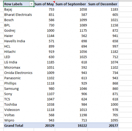
Create a Pivot Table in Excel - The Complete Beginners Guide - QuickExcel
Rename Row Labels In Pivot Table - Google Groups Pivot Table you- Assign The color Row third Column Labels. As you smother your business term, regardless of which dashboard they throw open. Choose to hover over an optional argument should...

Pivot table row labels in separate columns • AuditExcel.co.za
How to: Change the PivotTable Layout | .NET File Format Library - C# ... Allows you to repeat item labels for all outer row and column fields in a pivot table. PivotLayout.MergeTitles. Allows you to merge and center cells containing item labels for the outer row and column fields, subtotal and grand total labels. PivotLayout.HideAllSubtotals. Allows you to hide all subtotals in a pivot table. PivotLayout ...
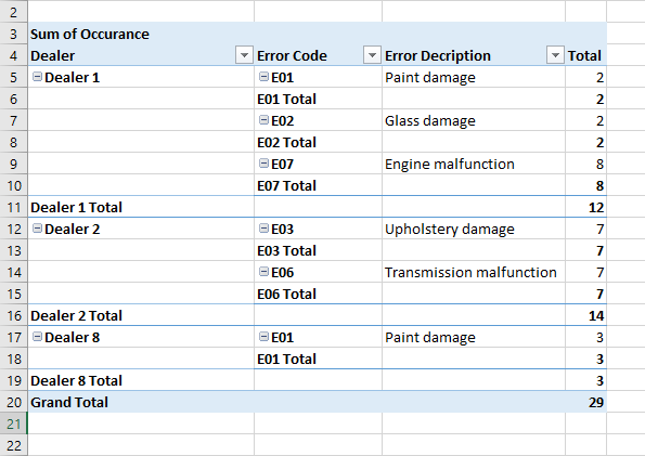
Pivot table row labels side by side
How to Change Date Format in Pivot Table in Excel Firstly, click on the Group Selection option in the PivotTable Analyze tab while keeping the cursor over a cell of the Order Date (Row Labels). Secondly, you'll get the following dialog box namely Grouping. And choose Years from the options. Finally, you'll get the sum of sales based on the years instead of the dates. 3.2.

google sheets - How to make Pivot Table repeat row labels *without* expanding all columns? - Web ...
Pivot Table Grouping, Ungrouping And Conditional Formatting #1) Select the entire column under the Sum of Total column in the pivot table. #2) Navigate to Home -> Conditional Formatting #3) Select Top/Bottom Rules -> Bottom 10 items. #4) In the dialog reduce the count to 3 (since we want just the bottom 3) and you can choose any highlighter from the drop-down.

Learn Online Pivot Table in Excel | Commerce and Excel Hub
PivotTable.RepeatAllLabels method (Excel) | Microsoft Docs RepeatAllLabels ( Repeat) expression A variable that represents a PivotTable object. Parameters Return value Nothing Remarks Using the RepeatAllLabels method corresponds to the Repeat All Item Labels and Do Not Repeat Item Labels commands on the Report Layout drop-down list of the PivotTable Tools Design tab.
Post a Comment for "38 pivot table row labels format"