39 how to show alternate data labels in excel
› blog › 2021A Comprehensive guide to Microsoft Excel for Data Analysis Nov 24, 2021 · You can make a chart, modify its type, adjust the row or column, the legend location, and the data labels. Column Chart, Line Chart, Pie Chart, Bar Chart, Area Chart, Scatter Plot are some of the different types of charts provided in Microsoft Excel. 10) Data Validation. Only valid values may need to be entered into cells. Drop-down List Arrow Always Visible in Excel - Excel Campus Here are the steps to create the icon: Select the cell to the right of the cell that contains a validation list. Go to the Insert tab on the ribbon, press the Symbol button. On the Symbol window, choose " Wingdings 3 " from the Text drop-down. Find the symbol that looks like the down-arrow.
› combination-clustered-andCombination Clustered and Stacked Column Chart in Excel There are actually several approaches to create a combined clustered and stacked chart in Excel. The approach demonstrated in this example keeps the underlying source data structured in a readable format. The alternate approach involves structuring the data with many extra blank cells sprinkled throughout the data.

How to show alternate data labels in excel
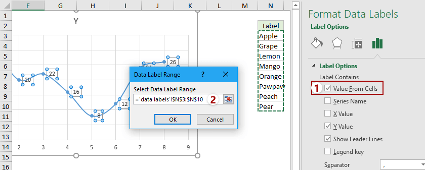
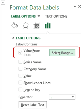
how to add data labels into Excel graphs - storytelling with data Let's look now at an alternative approach: embedding the labels directly. You can download the corresponding Excel file to follow along with these steps: Right-click on a point and choose Add Data Label. You can choose any point to add a label—I'm strategically choosing the endpoint because that's where a label would best align with my design. Add or remove data labels in a chart - support.microsoft.com Right-click the data series or data label to display more data for, and then click Format Data Labels. Click Label Options and under Label Contains , select the Values From Cells checkbox. When the Data Label Range dialog box appears, go back to the spreadsheet and select the range for which you want the cell values to display as data labels. Excel charts: add title, customize chart axis, legend and data labels ... Click anywhere within your Excel chart, then click the Chart Elements button and check the Axis Titles box. If you want to display the title only for one axis, either horizontal or vertical, click the arrow next to Axis Titles and clear one of the boxes: Click the axis title box on the chart, and type the text.
How to show alternate data labels in excel. Edit titles or data labels in a chart - support.microsoft.com The first click selects the data labels for the whole data series, and the second click selects the individual data label. Right-click the data label, and then click Format Data Label or Format Data Labels. Click Label Options if it's not selected, and then select the Reset Label Text check box. Top of Page Stagger long axis labels and make one label stand out in an Excel ... This is hard for the viewer to read. The common approach to solving this issue is to add a New Line character at the start of every second axis label by pressing Alt+Enter at the start of the label text or by using a formula to add CHAR(10) [the New Line character] at the start of the text (described well by Excel MVP Jon Peltier here).The method also involves forcing Excel to use every label ... › sort-by-color-in-excelSort by color in Excel (Examples) | How to Sort data with Color? In Excel, there are two ways to sort any data by Color. Firstly, we can sort the data by color through filters. For this, apply the filter selecting an option from the Data menu tab and then select the Sort by cell color or font color from the drop-down option. And other ways is sorting the data using the Sort option available in the Data menu tab. How to Add Alternative Text to an Object in Microsoft Excel To add alt text to an object in Excel, open your spreadsheet, add an object (Insert > Picture), and then select the object. Right-click the object and then select "Edit Alt Text" from the menu that appears. Alternatively, you can select the "Alt Text" option in the "Accessibility" group of the "Picture Format" tab.
Apply Custom Data Labels to Charted Points - Peltier Tech Click once on a label to select the series of labels. Click again on a label to select just that specific label. Double click on the label to highlight the text of the label, or just click once to insert the cursor into the existing text. Type the text you want to display in the label, and press the Enter key. How to AutoFit in Excel: adjust columns and rows to match data size To AutoFit column width, select one, several or all columns on the sheet, go to the Home tab > Cells group, and click Format > AutoFit Column Width. To AutoFit row height, select the row (s) of interest, go to the Home tab > Cells group, and click Format > AutoFit Row Height. AutoFit column width and row height using a keyboard shortcut Format Data Label Options in PowerPoint 2013 for Windows Alternatively, select data labels of any data series in your chart and right-click to bring up a contextual menu, as shown in Figure 2, below.From this menu, choose the Format Data Labels option.; Figure 2: Format Data Labels option Either of these options opens the Format Data Labels Task Pane, as shown in Figure 3, below.In this Task Pane, you'll find the Label Options and Text Options tabs. Add Custom Labels to x-y Scatter plot in Excel Step 1: Select the Data, INSERT -> Recommended Charts -> Scatter chart (3 rd chart will be scatter chart) Let the plotted scatter chart be Step 2: Click the + symbol and add data labels by clicking it as shown below. Step 3: Now we need to add the flavor names to the label. Now right click on the label and click format data labels.
How to Change Excel Chart Data Labels to Custom Values? Define the new data label values in a bunch of cells, like this: Now, click on any data label. This will select "all" data labels. Now click once again. At this point excel will select only one data label. Go to Formula bar, press = and point to the cell where the data label for that chart data point is defined. › dynamically-labelDynamically Label Excel Chart Series Lines • My Online ... Step 1: Duplicate the Series. The first trick here is that we have 2 series for each region; one for the line and one for the label, as you can see in the table below: Select columns B:J and insert a line chart (do not include column A). To modify the axis so the Year and Month labels are nested; right-click the chart > Select Data > Edit the ... Excel Charts: Creating Custom Data Labels - YouTube Description. In this video I'll show you how to add data labels to a chart in Excel and then change the range that the data labels are linked to. This video covers both Windows and Mac versions of ... Add second x axis to Excel 2016 - Microsoft Tech Community Mixed Reality. Enabling Remote Work. Small and Medium Business. Humans of IT. Empowering technologists to achieve more by humanizing tech. Green Tech. Raise awareness about sustainability in the tech sector. MVP Award Program. Find out more about the Microsoft MVP Award Program.
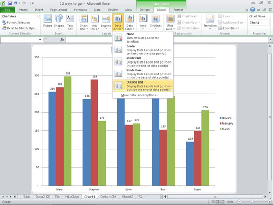
Microsoft Tips with Temo!: How to Add Data Labels to an Excel 2010 Chart
› blog › create-sunburst-chartCreate an Excel Sunburst Chart With Excel 2016 - MyExcelOnline Jul 22, 2020 · STEP 5: Go to Chart Design > Add Chart Element > Data Labels > More Data Label Options. STEP 6: In the Format Data Labels dialog box, Check the Value box. Value will be displayed next to the category name: Now that you have learned how to create a Sunburst Chart in Excel, let’s move forward and know about the advantages and disadvantages of ...
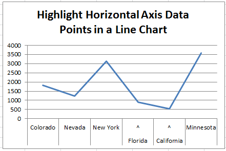
How-to Highlight Specific Horizontal Axis Labels in Excel Line Charts
Excel tutorial: How to customize axis labels Now let's customize the actual labels. Let's say we want to label these batches using the letters A though F. You won't find controls for overwriting text labels in the Format Task pane. Instead you'll need to open up the Select Data window. Here you'll see the horizontal axis labels listed on the right. Click the edit button to access the ...
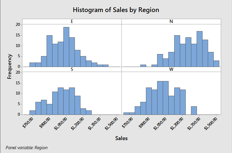
5 Minitab graphs tricks you probably didn’t know about - Master Data Analysis
Custom data labels in a chart - Get Digital Help Press with right mouse button on on any data series displayed in the chart. Press with mouse on "Add Data Labels". Press with mouse on Add Data Labels". Double press with left mouse button on any data label to expand the "Format Data Series" pane. Enable checkbox "Value from cells".
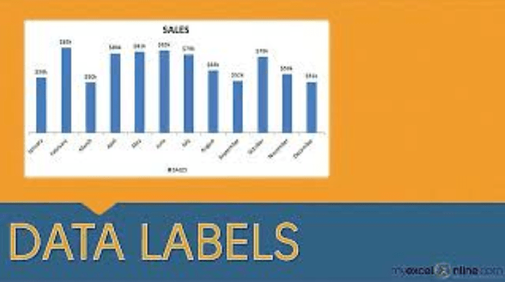
Adding Data Labels To An Excel Chart | Free Microsoft Excel Tutorials
Excel Chart Vertical Axis Text Labels - My Online Training Hub Hide the left hand vertical axis: right-click the axis (or double click if you have Excel 2010/13) > Format Axis > Axis Options: Set tick marks and axis labels to None; While you're there set the Minimum to 0, the Maximum to 5, and the Major unit to 1. This is to suit the minimum/maximum values in your line chart.
30 What Is A Data Label In Excel - Labels Database 2020
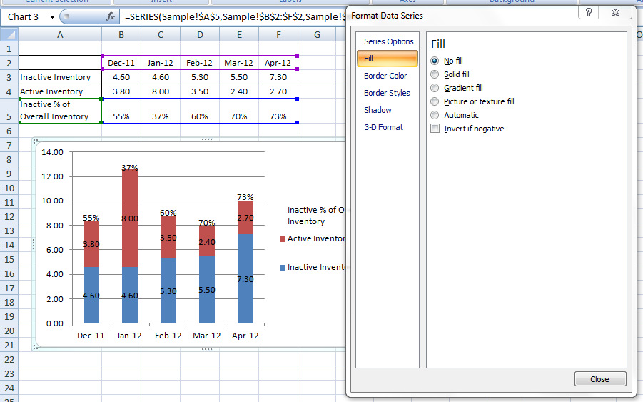
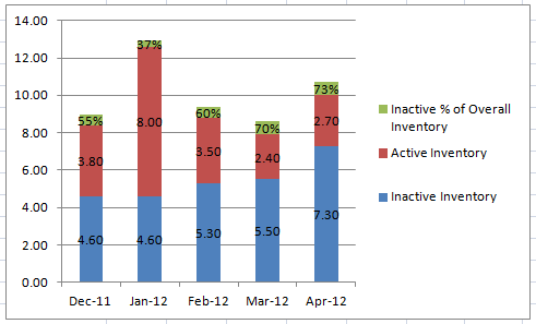
› year-on-year-chartsYear on Year Charts • My Online Training Hub Another option is to show the variance year on year, but this only works well for two years’ worth of data. The chart below clearly shows the comparison year on year with the current year at the front in a bright attention grabbing colour. Data labels add another layer of information that is quick and easy to interpret.

E-xcel Tuts: Add Data Labels to Excel Charts
How to add data labels from different column in an Excel chart? This method will guide you to manually add a data label from a cell of different column at a time in an Excel chart. 1. Right click the data series in the chart, and select Add Data Labels > Add Data Labels from the context menu to add data labels. 2. Click any data label to select all data labels, and then click the specified data label to select it only in the chart.
Excel Dashboard Templates How-to Put Percentage Labels on Top of a Stacked Column Chart - Excel ...
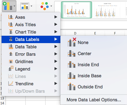
How to Add Data Labels to an Excel 2010 Chart - dummies Excel provides several options for the placement and formatting of data labels. Use the following steps to add data labels to series in a chart: Click anywhere on the chart that you want to modify. On the Chart Tools Layout tab, click the Data Labels button in the Labels group. A menu of data label placement options appears: None: The default choice; it means you don't want to display data labels. Center to position the data labels in the middle of each data point. Inside End to position the ...

How To Use Dynamic Data Labels To Create Interactive Excel Charts
Make your Excel charts easier to read with custom data labels make up an Excel graph. But if the data labels are not at the correct data ... and clear the Show Legend check box. Click the Data Labels tab and, in the Label Contains section, click the Value ...

Merge Mailing Labels Word 2003
Stagger Axis Labels to Prevent Overlapping - Peltier Tech Alternatively, in the Format Axis task pane, select Text Options, then click on the Textbox icon, then where the Custom Angle box is blank, enter any nonzero value, then enter zero. I don't know why you need to do either thing twice, but Excel is like that sometimes. Now the labels are horizontal.
How to set and format data labels for Excel charts in C#
› analyze-large-data-setsExcel for Commerce | Analyze large data sets in Excel May 07, 2015 · You can see that the row labels at the left of the screen only show the rows in which ‘Aaliah’ appears in the Name column. You can filter on multiple conditions in a column (for example, ‘Aaliah’ and ‘Aaliya’ in the Name column) and/or filter using multiple columns (for example, only certain years).
How-to Put Percentage Labels on Top of a Stacked Column Chart - Excel Dashboard Templates
Column chart skips every other month on x-axis - Power BI Select your Date field in Fieds tab and set the format as Month, Year in Formatting options ( Modelling -> Formating). Thanks Raj Message 4 of 5 14,869 Views 1 Reply wcurtis Frequent Visitor In response to rajendran 07-09-2018 10:01 AM Raj, Yes, that works perfectly, Thank you!!!! Message 5 of 5 14,764 Views 0 Reply
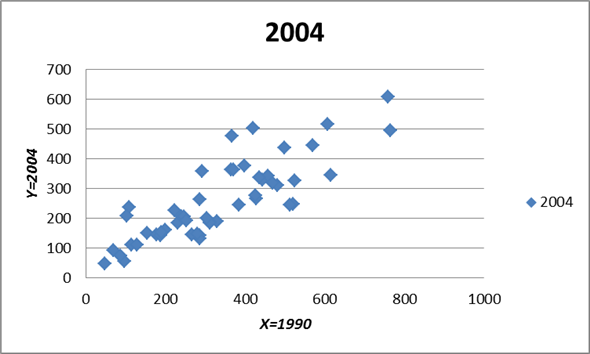
Solved: (a) Make an Excel scatter plot of X = 1990 assault rate... | Chegg.com
How to show different fonts for different data labels ... - Stack Overflow import pandas as pd import xlsxwriter # initialize list of lists data = [ ['tom', 10], ['jerry', 15], ['julie', 14], ['amy', 12], ['tony', 13]] # create pandas df df_new = pd.dataframe (data, columns = ['name', 'apples']) # write everything to an excel file writer = pd.excelwriter ('./test.xlsx', engine='xlsxwriter') df_new.to_excel (writer, …
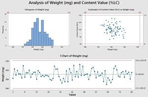
5 Minitab graphs tricks you probably didn’t know about - Master Data Analysis
How to display different text than the value in same cell? 1. Select the cell values that you want to display them with different text, and then click Home > Conditional Formatting > New Rule, see screenshot: 2. Then in the New Formatting Rule dialog box, click Use a formula to determine which cells to format under the Select a Rule Type list box, and then enter this formula: =c1=1 ( C1 is the first cell ...
How to Make Charts and Graphs in Excel | Smartsheet
Chart: Display alternative values as Data Labels or Data Callouts If A2:A50000 contain data. Enter a formula in B2. Select B2. Double-click the Fill Handle and Excel will shoot the formula down to B50000.
Show Trend Arrows in Excel Chart Data Labels
Create Dynamic Chart Data Labels with Slicers - Excel Campus You basically need to select a label series, then press the Value from Cells button in the Format Data Labels menu. Then select the range that contains the metrics for that series. Click to Enlarge Repeat this step for each series in the chart. If you are using Excel 2010 or earlier the chart will look like the following when you open the file.

30 How To Add Label To Excel Chart - Labels Database 2020
Display every "n" th data label in graphs - Microsoft Community Change the step value (the on in bold) as required Sub PointLabel () Dim mySrs As Series Dim iPts As Long If ActiveChart Is Nothing Then MsgBox "Select a chart and try again.", vbExclamation, "No Chart Selected" Else For Each mySrs In ActiveChart.SeriesCollection With mySrs For iPts = 1 To .Points.count Step 5 ' add label

How to Add Data Labels in Excel - Excelchat | Excelchat
Excel charts: add title, customize chart axis, legend and data labels ... Click anywhere within your Excel chart, then click the Chart Elements button and check the Axis Titles box. If you want to display the title only for one axis, either horizontal or vertical, click the arrow next to Axis Titles and clear one of the boxes: Click the axis title box on the chart, and type the text.
Post a Comment for "39 how to show alternate data labels in excel"