43 row labels in excel pivot table
Repeat item labels in a PivotTable - support.microsoft.com Right-click the row or column label you want to repeat, and click Field Settings. Click the Layout & Print tab, and check the Repeat item labels box. Make sure Show item labels in tabular form is selected. Notes: When you edit any of the repeated labels, the changes you make are applied to all other cells with the same label. How do you add labels to a pivot table in Excel? Add data labels Click the chart, and then click the Chart Design tab. Click Add Chart Element and select Data Labels, and then select a location for the data label option. Note: The options will differ depending on your chart type. If you want to show your data label inside a text bubble shape, click Data Callout.
Sorting to your Pivot table row labels in custom order [quick tip] Create a pivot table with data set including sort order column. Add sort order column along with classification to the pivot table row labels area. Add the usual stuff to values area. Set up pivot table in tabular layout. Remove sub totals Finally hide the column containing sort order. Your new pivot report is ready.
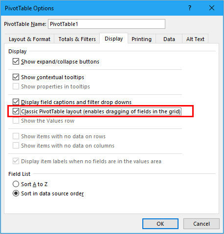
Row labels in excel pivot table
How to make row labels on same line in pivot table? Make row labels on same line with PivotTable Options You can also go to the PivotTable Options dialog box to set an option to finish this operation. 1. Click any one cell in the pivot table, and right click to choose PivotTable Options, see screenshot: 2. How to Use Excel Pivot Table Label Filters - Contextures Excel Tips In an Excel pivot table, you might want to hide one or more of the items in a Row field or Column field. To do that, you could click the drop down arrow for the Row or Column Labels, to see the list of pivot items in that pivot field. Then, in the list, remove the check mark for items you want to remove. get a row label from pivot table - Microsoft Tech Community Creating PivotTable add data to data model by checking Create PivotTable and after that convert it to cube formulas. Now you may take these formulas and convert it to form you need, for example in H3 it could be =CUBEVALUE( "ThisWorkbookDataModel", CUBEMEMBER("ThisWorkbookDataModel", " [Measures].
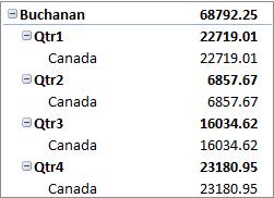
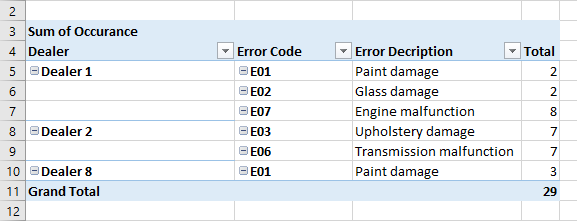
Row labels in excel pivot table. Pivot Table "Row Labels" Header Frustration - Microsoft Community Hub Pivot Table "Row Labels" Header Frustration. Janie1964. Occasional Visitor. Jul 28 2021 12:03 PM. Design the layout and format of a PivotTable To change the layout of a PivotTable, you can change the PivotTable form and the way that fields, columns, rows, subtotals, empty cells and lines are displayed. To change the format of the PivotTable, you can apply a predefined style, banded rows, and conditional formatting. Windows Web Mac Changing the layout form of a PivotTable Pivot table row labels side by side - Excel Tutorial - OfficeTuts Excel You can copy the following table and paste it into your worksheet as Match Destination Formatting. Now, let's create a pivot table ( Insert >> Tables >> Pivot Table) and check all the values in Pivot Table Fields. Fields should look like this. Right-click inside a pivot table and choose PivotTable Options…. Check data as shown on the image below. Pivot Table Row Labels - Microsoft Community If you go to PivotTable Tools > Analyze > Layout > Report Layout > Show in Tabular Form, your column headers will be used for the row labels. Every once in a while there's a sudden gust of gravity... Report abuse 1 person found this reply helpful · Was this reply helpful? Yes No A. User Replied on December 19, 2017
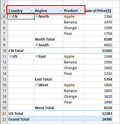
How to make row labels on same line in pivot table? - ExtendOffice Make row labels on same line with PivotTable Options You can also go to the PivotTable Options dialog box to set an option to finish this operation. 1. Click any one cell in the pivot table, and right click to choose PivotTable Options, see screenshot: 2. Group or ungroup data in a PivotTable - support.microsoft.com Group or ungroup data in a PivotTable. Excel for Microsoft 365 Excel for Microsoft 365 for Mac More... Grouping data in a PivotTable can help you show a subset of data to analyze. For example, you may want to group an unwieldy list date and time fields in the PivotTable into quarters and months. Windows Mac. Automatic Row And Column Pivot Table Labels - How To Excel At Excel The first thing to do is put your cursor somewhere in your data list Select the Insert Tab Hit Pivot Table icon Next select Pivot Table option Select a table or range option Select to put your Table on a New Worksheet or on the current one, for this tutorial select the first option Click Ok Data Labels in Excel Pivot Chart (Detailed Analysis) Add a Pivot Chart from the PivotTable Analyze tab. Then press on the Plus right next to the Chart. Next open Format Data Labels by pressing the More options in the Data Labels. Then on the side panel, click on the Value From Cells. Next, in the dialog box, Select D5:D11, and click OK.
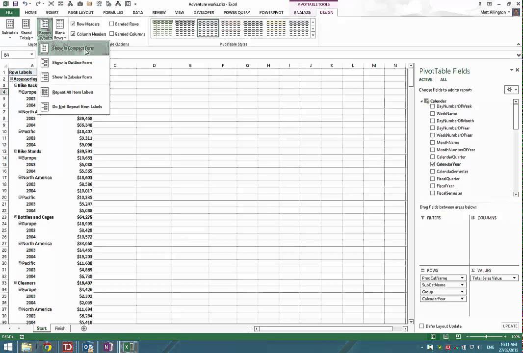
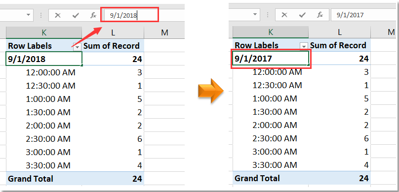
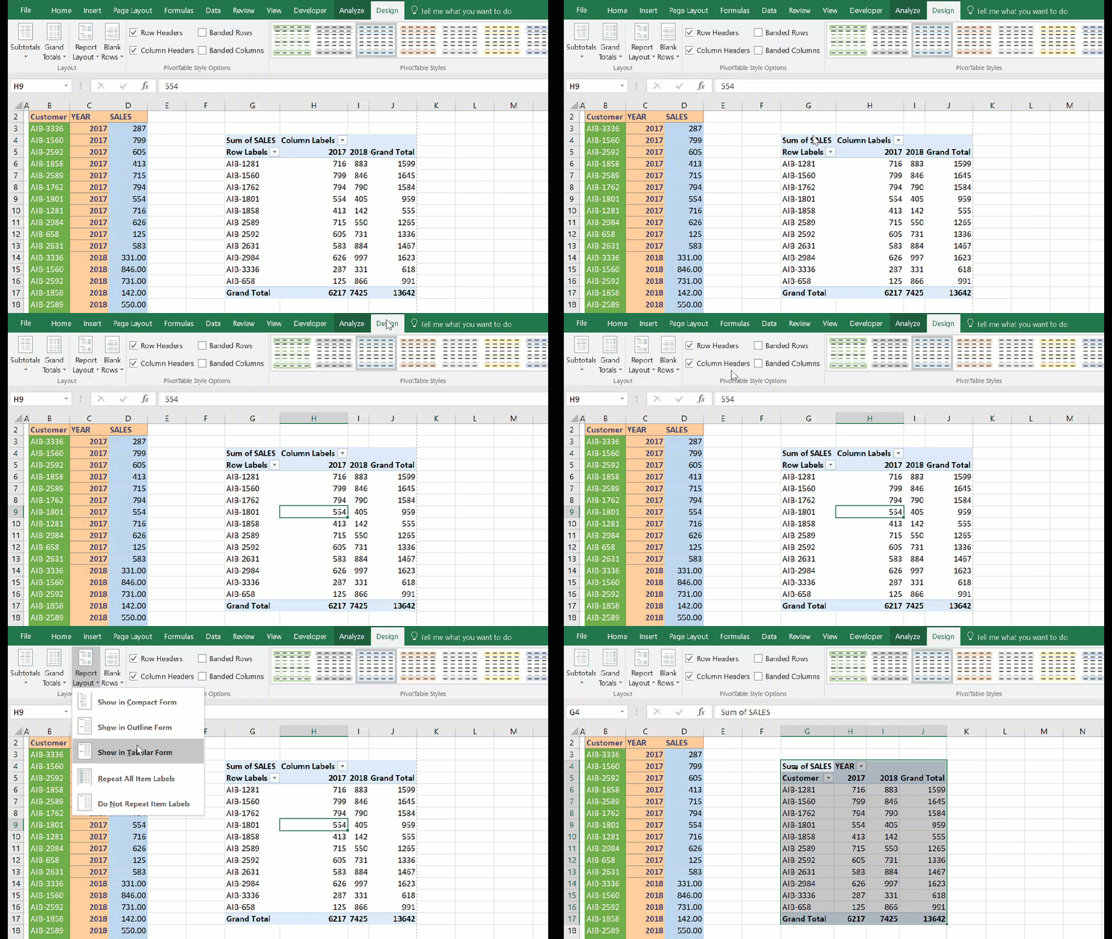
How to Flatten Data in Excel Pivot Table? - GeeksforGeeks Select a range that you want to flatten - typically, a column of labels. Highlight the empty cells only - hit F5 (GoTo) and select Special > Blanks. Type equals (=) and then the Up Arrow to enter a formula with a direct cell reference to the first data label. Instead of hitting enter, hold down Control and hit Enter. Pivot table row labels in separate columns • AuditExcel.co.za Our preference is rather that the pivot tables are shown in tabular form (all columns separated and next to each other). You can do this by changing the report format. So when you click in the Pivot Table and click on the DESIGN tab one of the options is the Report Layout. Click on this and change it to Tabular form. How to rename group or row labels in Excel PivotTable? - ExtendOffice To rename Row Labels, you need to go to the Active Field textbox. 1. Click at the PivotTable, then click Analyze tab and go to the Active Field textbox. 2. Now in the Active Field textbox, the active field name is displayed, you can change it in the textbox. How to make row labels on same line in pivot table in excel #ExcelMaster, #PivotTable, #ExcelHow to make row labels on same line in pivot table in excelHow to show multiple rows in pivot table in excel
How to make row labels on same line in pivot table?
Change row label in Pivot Table with VBA | MrExcel Message Board If they are row labels they do not appear as columns, they would be column fields/labels. If they appear as columns they are not row labels. If you want to change a field name between the source table and the pivot table I suggest you do this in SQL. So if the source data has fields Type and Manufacturer but you want them to be Type and Country ...

Pivot table row labels side by side – Excel Tutorial
How to repeat row labels for group in pivot table? - ExtendOffice Except repeating the row labels for the entire pivot table, you can also apply the feature to a specific field in the pivot table only. 1. Firstly, you need to expand the row labels as outline form as above steps shows, and click one row label which you want to repeat in your pivot table. 2.
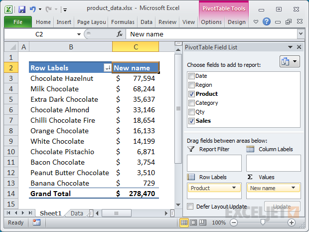
Pivot Table Tips | Exceljet
get a row label from pivot table - Microsoft Tech Community Creating PivotTable add data to data model by checking Create PivotTable and after that convert it to cube formulas. Now you may take these formulas and convert it to form you need, for example in H3 it could be =CUBEVALUE( "ThisWorkbookDataModel", CUBEMEMBER("ThisWorkbookDataModel", " [Measures].
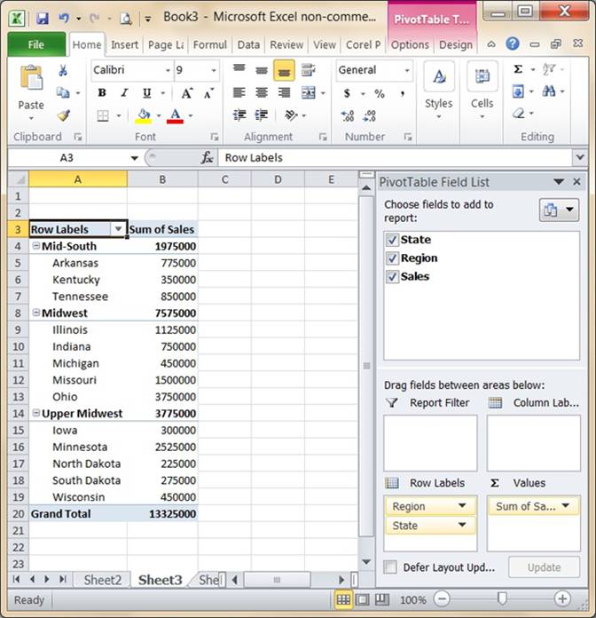
Excel PivotTable Percentage: Which Customers Are Costing You ...
How to Use Excel Pivot Table Label Filters - Contextures Excel Tips In an Excel pivot table, you might want to hide one or more of the items in a Row field or Column field. To do that, you could click the drop down arrow for the Row or Column Labels, to see the list of pivot items in that pivot field. Then, in the list, remove the check mark for items you want to remove.
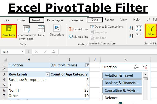
Pivot Table Filter in Excel | How to Filter Data in a Pivot ...
How to make row labels on same line in pivot table? Make row labels on same line with PivotTable Options You can also go to the PivotTable Options dialog box to set an option to finish this operation. 1. Click any one cell in the pivot table, and right click to choose PivotTable Options, see screenshot: 2.
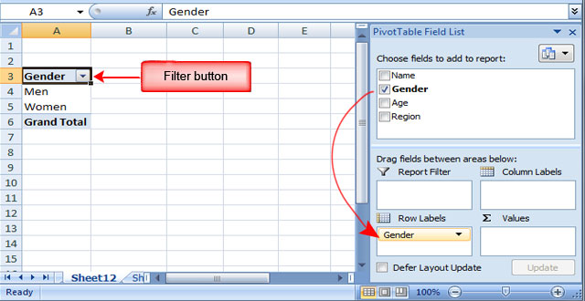
Lesson 54: Pivot Table Row Labels - Swotster
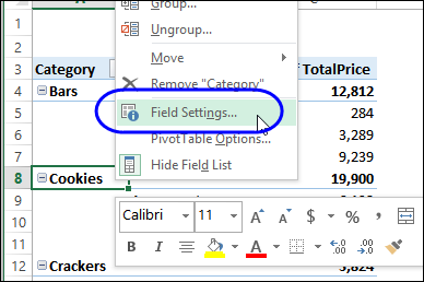
Turn Repeating Item Labels On and Off | Excel Pivot Tables

Change Pivot Table Sum of Headings and Blank Labels - YouTube
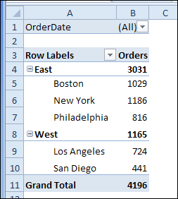
Repeat Pivot Table Labels in Excel 2010 | Excel Pivot Tables
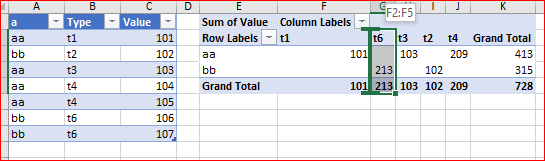
Manually Sorting Pivot Table Columns - Microsoft Community Hub

Microsoft Excel – showing field names as headings rather than ...
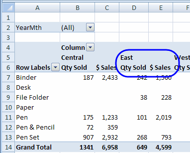
Centre Column Headings in Excel Pivot Table | Excel Pivot Tables
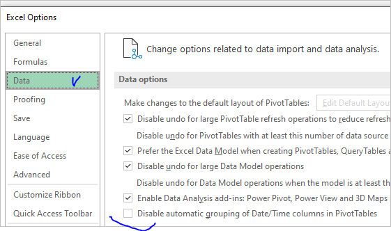
Pivot table manual row label filter no longer allows expand ...
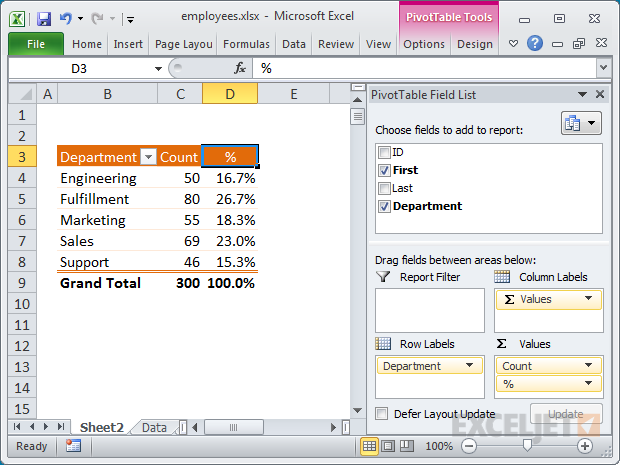
Pivot Table Tips | Exceljet

Pivot Table column label from horizontal to vertical ...

How to Use Label Filters for Text in the Pivot Table? - MS ...
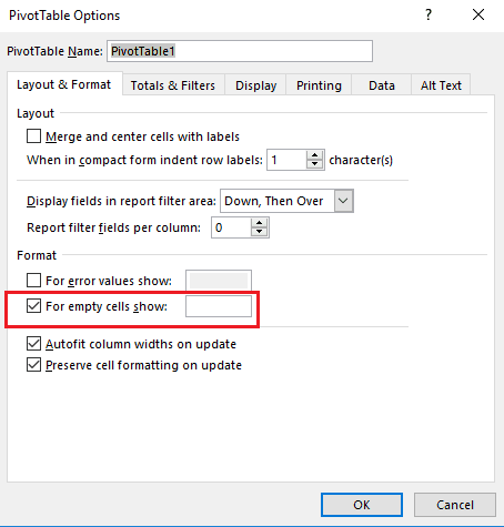
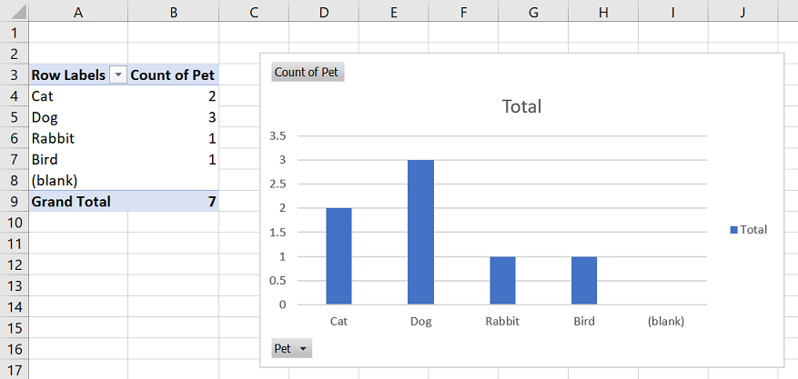
How To Remove (blank) Values in Your Excel Pivot Table - MPUG
Design the layout and format of a PivotTable
Add Multiple Columns to a Pivot Table | CustomGuide

Pivot table row labels in separate columns • AuditExcel.co.za
Pivot table row labels side by side – Excel Tutorial

Microsoft Excel – showing field names as headings rather than ...

Repeat Pivot Table row labels • AuditExcel.co.za Pivot Tables ...

Fix Excel Pivot Table Missing Data Field Settings
How to make row labels on same line in pivot table?
Excel 2016 – How to exclude (blank) values from pivot table
How to Flatten and repeat Row Labels in a Pivot Table
Change Blank Labels in a Pivot Table – Contextures Blog

Pivot table row labels side by side – Excel Tutorial
MS Excel 2013: Display the fields in the Values Section in a ...
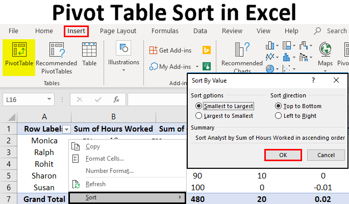
Pivot Table Sort in Excel | How to Sort Pivot Table Columns ...

Automatic Row And Column Pivot Table Labels
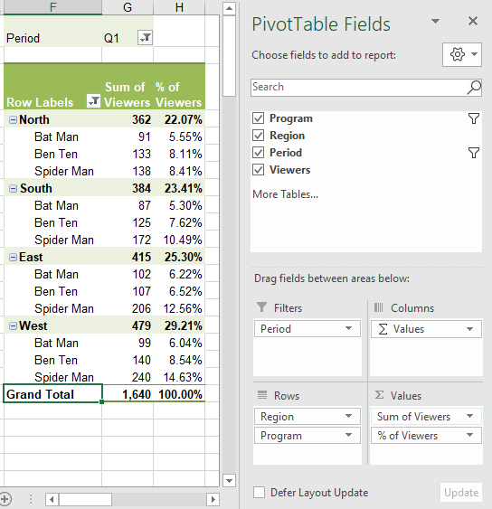
Excel Pivot Tables Explained • My Online Training Hub
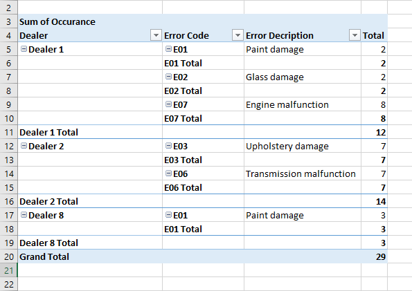
Pivot table row labels side by side – Excel Tutorial

Remove filter from ROW LABELS on pivot table Excel - Super User

Pivot table row labels in separate columns • AuditExcel.co.za

Pivot Tables Row Labels in Excel 2007 - YouTube
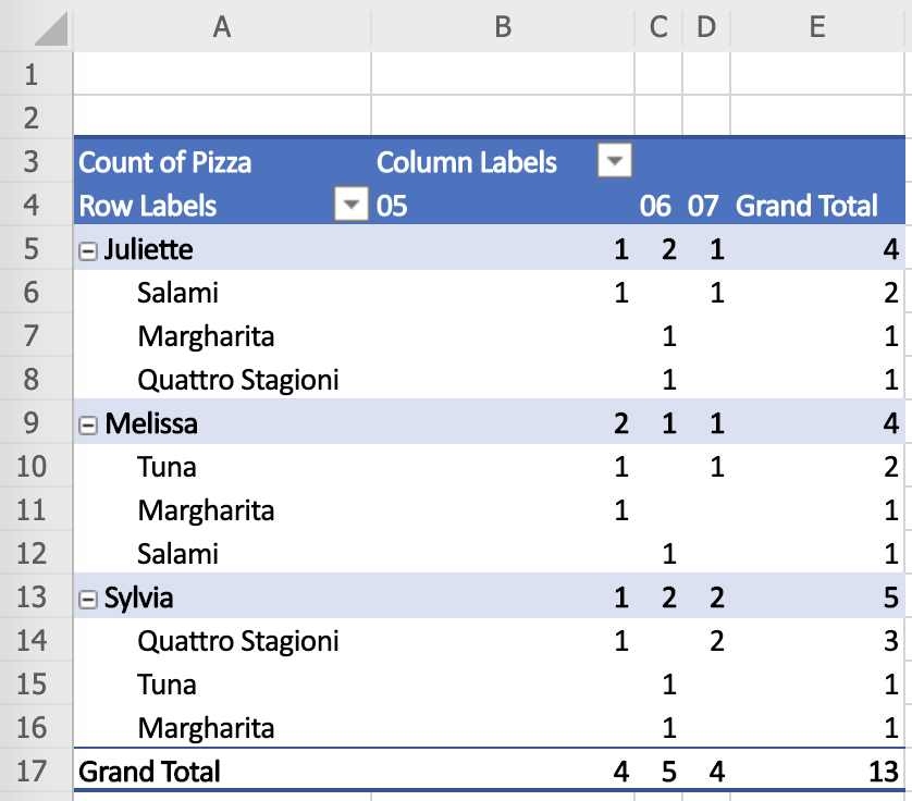
What is a Pivot Table & How to Create It? Complete 2022 Guide ...

Removing old Row and Column Items from the Pivot Table ...

Excel pivot table shows only when rows have multiple other ...
How to rename group or row labels in Excel PivotTable?

Excel 2007 Pivot Tables- Column labels can do everything row labels can do- same in latest versions
Automatic Row And Column Pivot Table Labels
Post a Comment for "43 row labels in excel pivot table"